What happens if someone presents a new data trace without any contextual information and asks you to do a quick peak check by eye?
In most of the cases we are simply searching for ...
PEAK is doing exactly the same. In the first step PEAK determines all inflexion points (see 8) and the corresponding y-axis distance (see 10) to their direct predecessor. If this distance exceeds a certain threshold (see 11) the currently regarded inflexion point will be marked as peak tip (see 9) and its direct predecessor and successor as peak start and end, respectively.
The threshold for each single inflexion point is individually derived from its corresponding neighborhood. Thereby, the neighborhood radius (see 27) determines how many inflexion point distances before (neighborhood A) and after (neighborhood B) the currently regarded inflexion point will be taken into account. Finally, both neighborhoods are combined to a single reference value by calculating the individual median or mean (see 21) and selecting the maximum or minimum (see 22) from both values. This value multiplied by the user-defined significance factor (see 28) has to be exceeded by the y-axis distance of the currently regarded inflexion point in order to be outstanding within its direct neighborhood and thus a real peak.
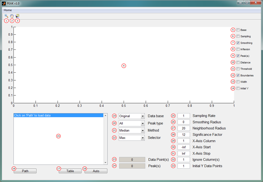
01: Zoom data in / out.
02: Move plotted data trace.
03: Data cursor
04: Data visualization area
05: Plot data base (see 19).
06: Plot sampling result (see 25).
07: Plot smoothing result (see 26).
08: Plot inflexion points.
09: Plot detected peak tips.
10: Plot inflexion point distances.
11: Plot peak thresholds.
12: Plot peak start and end.
13: Plot half-maximum peak width.
14: Mark initial Y value data base (see 33).
15: Data browser
For each valid data file the data browser contains the file name and
file size (in squared brackets) followed by the corresponding sweep and column numbers.
Invalid data files get automatically skipped.
16: Click to choose the data path.
Each file in the selected path and all its subfolders will be scanned for processable information.
Valid data files are regular text files (e.g. *.txt, *.dat, *.asc) containing at least two
numeric data columns (x- and y-axis). Additional header lines or multiple sweeps within one
file are valid and handled automatically.
17: Click to generate a single Microsoft Excel result file for the currently analyzed data trace.
The result file includes beside the complete set of user-defined parameters (see 19-22 and
25-33) the following information for each data trace:
- File name
- Sweep number
- Column number
- Initial Y value
- Total number of peaks
- Interpeak interval (IPI)
- Peak height
- Half-maximum peak width
- Peak start (x and y coordinate)
- Peak tip (x and y coordinate)
- Peak end (x and y coordinate)
- Peak half-maximum (x1, x2 and y coordinate)
18: Click to generate a single Microsoft Excel result file of all data traces in the data browser.
During that process each single data trace in the data browser gets automatically selected and
analyzed based on the same set of parameters.
19: Switch between the original data trace and its derivative-like representation.
Selecting "Derivative" replaces each y-axis value by the y-axis distance to its
predecessor (ΔY) while the x-axis remains unaffected.
20: Filter results for a certain peak type.
Choose between "All", "Up" and "Down" to either detect all
kinds of peaks or filter for upward or downward peaks, respectively.
21: Choose between "Median" and "Mean" as operator during the neighborhood
evaluation.
An inflexion point is considered a peak tip if the distance to its nearest predecessor strongly differs from one of the two reference distances determined in its preceding and succeeding neighborhood (see 27). A reference distance is either the median or the mean of all inflexion point distances in the given neighborhood.
22: Select either the maximum or minimum from both neighborhood reference distances as comparison value.
The final peak judgement comprises the comparison of the current inflexion point distance with a multiple (significance factor, see 28) of one of the two neighborhood reference distances. This can be either the maximum ("Max") or minimum ("Min") of both values.
23: Total number of data points.
24: Total number of peaks.
25: Downsample data trace.
Consider only the first of x consecutive data points (x >= 1).
26: Smooth data trace by applying a sliding mean.
Replace every data point by the mean of itself, its x preceding and x succeeding data points (x >= 0).
27: Determine the total number of inflexion points per neighborhood.
While searching for outstanding peaks compare the current inflexion point with its x predecessors and x successors (x >= 1).
28: Significance factor
An outstanding peak is x times higher than its surrounding (x >= 1).
29: Use column x as x-axis (x >= 1).
30: Ignore all values before the x-axis value x (x ∈ [-∞,∞]).
31: Ignore all values after the x-axis value x (x ∈ [-∞,∞]).
32: Ignore specified columns x y z ... (x, y, z >= 1).
PEAK automatically ensures that at least two columns (x- and y-axis) remain.
33: Calculate the mean y-axis value of the first x data points (x >= 1).